Formatting Grids

General Overview

XLCubed Grid formatting is now controlled through the XLCubedformat sheet.

(For a grid which is static in shape, you can choose to manage formatting natively in Excel, and turn off XLCubed formatting. This is done by right clicking on the grid and in the properties menu, on the appearance tab, unchecking ‘Apply Formatting’.)

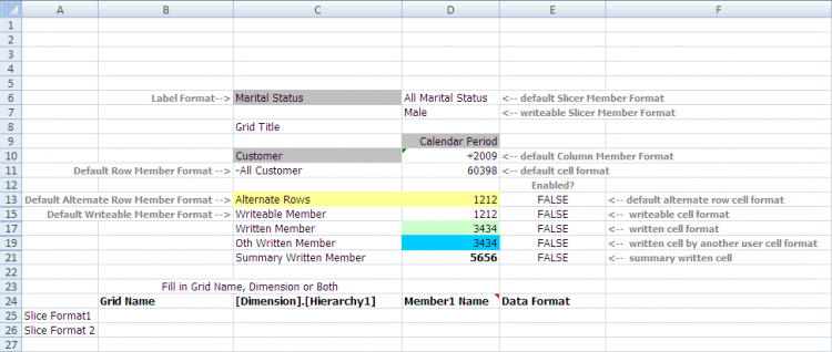
When the first XLCubed grid is inserted in a new workbook, the format sheet is copied in from the master format workbook. The format sheet can then be customised as required within this workbook. The default format sheet is shown below.

The layout is primarily that of a simple grid (C6:D21), with descriptions of each cell alongside. The format set in the Excel cell within this range is then applied to the corresponding area of the XLCubed grid when it is refreshed.

Where there is a requirement to format different grids in different ways, this is handled by the range A24:Exx.

Most common formatting requirements can be handled through the right click menu directly on an XLCubed grid, without any need to make changes directly on the format sheet. More complex requirements can be handled directly on the format sheet. When applying formatting through the right click menus, this will actually make the appropriate changes in the format sheet.

Right Click Formatting

The right click options available vary with whether you have selected a value, or a member name.

To apply a default numeric format to a grid: Use Excel to format the number as required, then right click the number and choose XLCubed – Formatting – Apply Format to Data. This sets the format of the selected cell as the default for all Measures (D11 on the XLCubedFormats sheet).

To apply differing formats to several measures: Open the member selector for ‘Measures’ (by double clicking the Measures hierarchy label, or right clicking the grid and choosing ‘Design Grid’ to open the report designer). Select the measures you wish to format, and then use the formatting button, highlighted below to set the Excel numeric format required for each measure.

This will apply the selected formats to the format sheet as shown below

Additional formats / background colours as required can then be applied to the member name and data format cells directly on the format sheet.

To format a Slice:

With a Dimension Member highlighted the following options are available, on the XLCubed – Formatting right click menu

• Apply Format to This Member – Choose this having first set the Excel cell formatting as required. The format is then applied to the member name and the data for this member.

• Select Number Format for This Member – This opens an Excel dialog to specify the number format for the data for the member selected.

• Apply Format to Column/Row Members - Choose this having first set the Excel cell formatting as required, and the format is then applied to all member names on rows or columns.

Each of these settings will add or amend a row in the format sheet from A25 onward, which can then be additionally changed as required directly on the format sheet.

Formatting directly through Format Sheet

More complex formatting scenarios or grid specific formatting are handled directly on the format sheet. Any of the cells on the format sheet can be formatted directly in Excel, and will then be applied to the appropriate are of the grid when the grid is next refreshed. The main body of the grid is contained in C6:D21, and the data cells, column and row member names, and the filter area can all be set directly here.

Alternate Rows: Alternate row formatting can be used by setting the drop down selector in E13 to ‘True’ and then applying the format required in C and D13. Writeback – Leaf Level: The grid can display the lowest level data and members in a specific format where required, by setting E15:21 to true as required.

Conditional Formatting: Conditional formatting on the grid data can be applied by setting the conditions on the default cell format (D11). This is currently only available at a grid level, and will become available at a slice level in version 6.1.

Grid Specific Formatting: Where multiple grids exist in a workbook, there may be a requirement to format a slice of data in a specific way in grid A, but not in grid B. Using the right click menus will apply the selected format to that slice of data in all grids. To make this grid specific, edit the format sheet and supply the grid name for the appropriate slice in column B. The example below in B26 is restricting the Bold formatting on CY 2004 to the ‘Sales’ grid, whereas the formatting on Germany is not restricted and will be applied on all grids.

When using this approach you must first name the grid, which is done in grid properties, on the appearance tab. Note that it’s also possible to use wildcards in the GridName field, so that for example all grids starting with Sales would apply this format (Sales*).

Slicer Formatting: XLCubed button slicers can be formatted as required in I5:Nxx.The font and button background can all be customised as required, and this can be achieved at an individual slicer level.

The image above shows the definition area in the format sheet, and a slicer which is formatted using this, in this case using the default format which had been set (1st row) rather than the custom entry for the GeographySlicer.

The formatting areas are:

Slicer Title: Only applicable when the ‘Show Title bar’ is checked in ‘Edit Slicer’ – settings tab. This applies back colour and font settings to the title.

Slicer Button: This applies back colour and font settings to the buttons, when they are in an unselected state

Slicer Button Selected: This applies back colour and font settings to the buttons, when they are in a selected state

Slicer Hover: This applies back colour and font settings to the buttons, when the mouse hovers over them.

Slicer Name: Populate this with the name of the slicer to create a customised format for a specific slicer. To name a slicer, go to Edit Slicer – settings tab.

Example - Grid Formatting

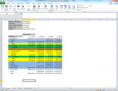
This grid report shows members at different levels in different background colours:

To achieve the row colouring as in the grid report above, we need to modify the XLCubedFormats sheet.

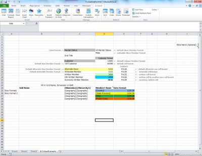
In the lower half of the XLCubedFormats sheet update the following columns:

• Dimension.Hierarchy - enter the dimension/hierarchy of the member that you wish to format. The Dimension/Hierarchy we wish to format is Geography. Note that you need to enclose in square brackets eg [Geography].[Geography].

• Member1 Name – enter the member name that you wish to format. Again enclose in square brackets. The member we wish to format is Country.

• Data format – this will determine the formatting for the grid data – in our example we are keeping the same format as for the Member, Country. You can choose to leave this blank – XLCubed formatting will then default to ‘default cell format’ (in the upper half of the XLCubedFormats sheet).

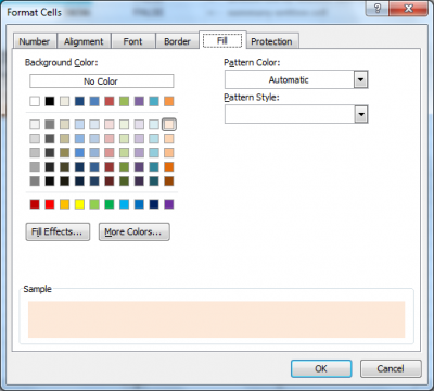
Next, using standard Excel formatting, change the fill-colour for [Country] and Data format to be blue.

We then have to include a separate entry for any other members we wish to format. We would also like to format at state level through to postal code. Repeat the same process for [State-Province], [City] and [Postal Code] each time choosing a different fill-colour. In our example we have chosen blue, yellow, green and orange.

Return to the grid worksheet and refresh the grid. You will find that the grid is formatted as:

• All country rows are coloured blue • All state rows are coloured yellow • All city rows are coloured green • All postal code rows are coloured orange

You will find that whenever you click on a row to expand it the formatting rules of the rows beneath will be as above.

Format Sheet Location and resetting

The default format sheet is specified under the Options menu on the ribbon XLCubed Options

This can be changed as required, for example to a network location to share customised corporate formats.

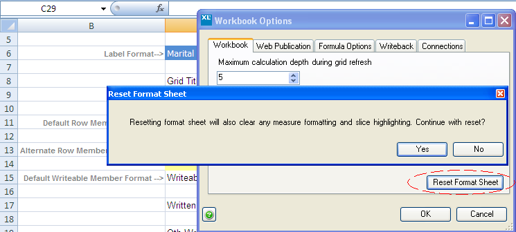
Should the Format Sheet need to be reset; use the Workbook Options to reset the Format Sheet in the current workbook to that held in the default path

Hiding the FormatSheet

By default, the format sheet will be visible in Excel. To hide the format sheet by default, use the XLCubed Options.